Useful Concepts in Machine Learning
Calibration of Models
When performing classification we often want not only to predict the class label, but also obtain a probability of the respective label. So after training a model, if this model is returning class labels and not returning the actual probabilities then we train a calibration moldel to calculate the probabilities.
- Using \(D_{train}\) learn a function \(f(x)\) and using \(D_{cross \ validation}: \{x_i, y_i\}\) create a table of values \(x_i, \hat{y_i}, y_i\), sorted in increasing order of \(\hat{y_i}\)
- Break the table into \(k\) chunks of size \(m\) and calculate \(mean \ y_i \ \forall \ j \ \epsilon \ k\) and call it \({y_{mean}^j}\) & \(mean \ \hat{y_i} \ \forall \ j \ \epsilon \ k\) and call it \({\hat{y}_{mean}^j}\) for each chunk
- \(D_{calibration} : \{\ \hat{y}_{mean}^j, y_{mean}^j \}\) , Calibration Plot : \(y_{axis} = y_{mean}^j, \ x_{axis} = \ \hat{y}_{mean}^j\)
- Now a Calibration function is trained to map \(\hat{y}_{mean}^j\) to \(y_{mean}^j\) (where \(y_{mean}^j\) is the probability if positive class)
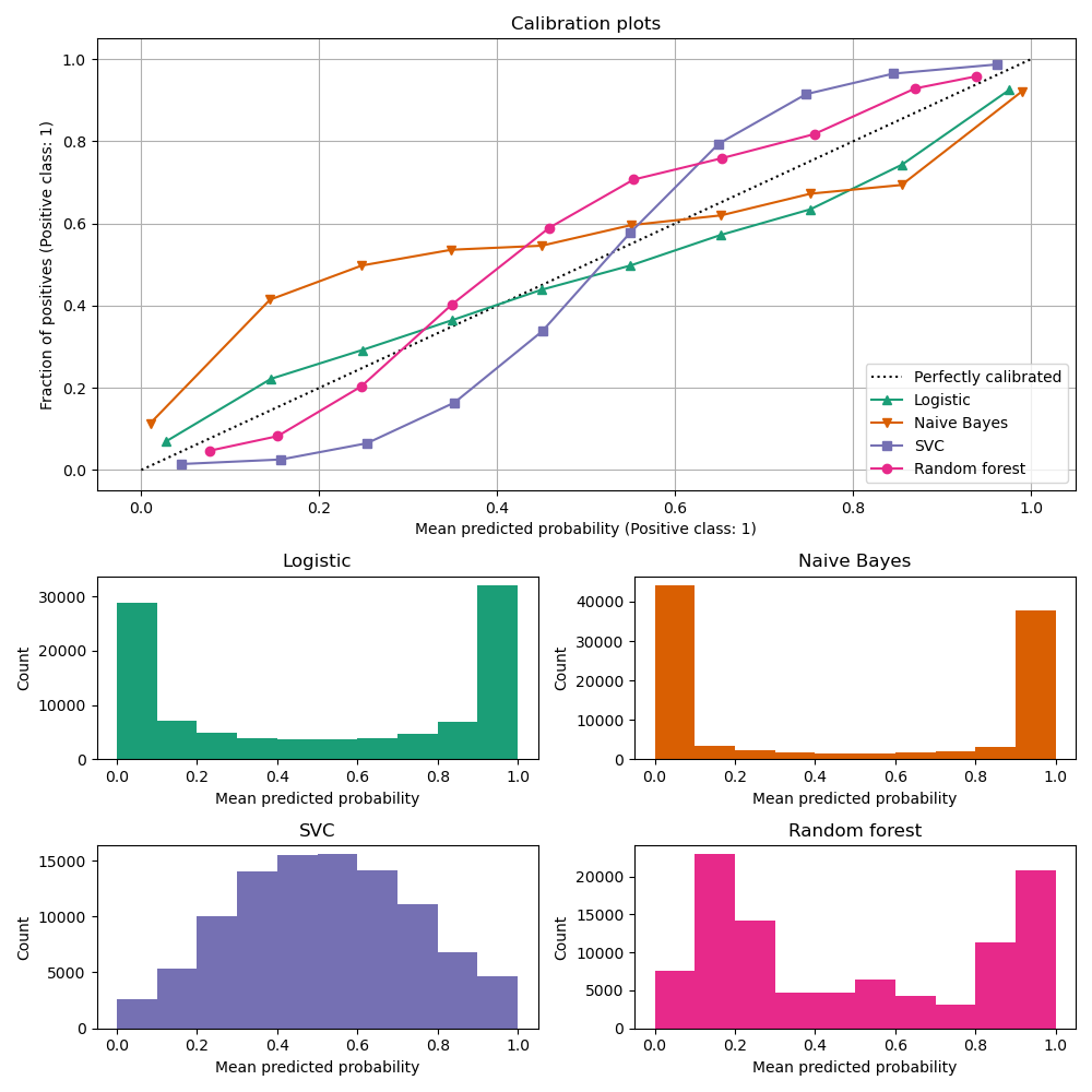 - Platt Scaling Callibration : Works only if the calibration plot looks like sigmoid
- Isotonic Regression Callibration : Learns Piece wise linear models, Works in almost all cases but needs more data than plat scaling
- CalibratedClassifierCV
- Probability calibration of classifiers
- Predicting Good Probabilities With Supervised Learning
- Platt Scaling Callibration : Works only if the calibration plot looks like sigmoid
- Isotonic Regression Callibration : Learns Piece wise linear models, Works in almost all cases but needs more data than plat scaling
- CalibratedClassifierCV
- Probability calibration of classifiers
- Predicting Good Probabilities With Supervised Learning
Random Sampling Consensus (RANSAC)
- Get a Random sample from \(D_{Train}\) call it \(D_0\) and build a Model \(M_0\) using \(D_0\)
- Compute outliers dataset \(O_o\) using abolute error based on the \(M_0\) prediction
- Now get the filtered data \(D_{train}^1 = D_{Train} - O_o\)
- Repeat the above steps to get \(D_{train}^2, D_{train}^3 ...\)
- When the \(M_i\) and \(M_{i+1}\) are very same then stop iterating and the \(M_{i+1}\) is a very robust model
Loss Minimisation Framework
Loss functions for classification
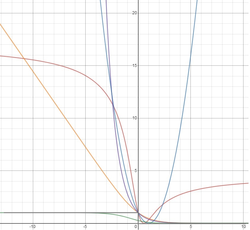
gray : Zero-one loss
green: Savage loss
orange: Logistic loss
purple: Exponential loss
brown: Tangent loss
blue: Square loss
- Logistic Regression : Logistic Loss (approximate of 0-1 loss) + Regulariser
- Linear Regression : Linear Loss + Regulariser
- SVM Regression : Hinge Loss + Regulariser
Hinge Loss : \(max(0, 1- y_i(w^Tx_i+b)) = \zeta_i\)
Overfitting, Underfitting, Variance, Bias and Generalisation
In general Overfitting results in High Variance Underfitting results in High Bias
If the data has high number of a constant value in prediction like : maximum 0s then Overfitting can result in High Bias
ToDo
- A/B Testing
- A-A-B Testing
- VC_dimension)